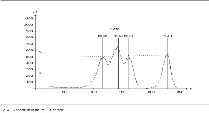
In questo quaderno sono raccolti alcuni esempi relativi alla spettroscopia alpha. In particolare sono state considerate le due run lunghe effettuate (nella camera a vuoto, usando come sorgente il $^{226}$Ra. Nella prima parte è stato acquisito direttamente il segnale proveniente dal preamp del fotodiodo, mentre nella seconda è stato inserito un attenuatore di rapporto $1:2$
In futuro vogliamo provare a terminare ad $1k\Omega$ in quanto il picco a dx risulta troppo stretto rispetto agli altri e non vi è un fondato motivo teorico.
Gli spettri sono da confrontare con
import matplotlib.pyplot as plt
import numpy as np
from scipy.optimize import curve_fit
nev, ts, qs, ql, ch = np.loadtxt("./DATI/datiPranzo.txt", unpack = True, skiprows = 1)
h, bins = np.histogram(ql, bins = 150)
binc = bins[:-1] + (bins[1]-bins[0])/2
%matplotlib inline
fig, ax = plt.subplots()
fig.set_size_inches(12,5)
ax.plot(binc, h, ds = "steps-mid", c = "darkgreen", lw = 2, label = "Spettro")
ax.fill_between(binc, h, step = "mid", color = "lime", alpha = 1)
#ax.plot(binc, myFun(binc, *popt))
ax.grid()
ax.set_xlabel("Energia [ADC]", fontsize = 14)
ax.set_ylabel("Entries", fontsize = 14)
ax.set_title("Dati pranzo", fontsize = 16)
ax.legend()
#ax.set_yscale("log")
plt.show()
%matplotlib inline
def gausLine(x,a,mu,sigma,m,q):
return a/(sigma*np.sqrt(2*np.pi)) * np.exp( -(x-mu)**2 / (2*sigma**2)) + m*x+q
startp0 = ( (100000, 1952, 50),
(100000, 2269, 50),
(100000, 2543, 50),
(100000, 3142, 20),)
startLine = (-3, 500)
myRange = ((1827,2049), (2187,2380), (2466,2634), (3039,3196))
lstPopt = []
lstPcov = []
def fitta(idx, ax):
cond = (binc > myRange[idx][0]) & (binc < myRange[idx][1])
xData = binc[cond]
yData = h[cond]
xDenso = np.linspace(xData.min(), xData.max(), num = 500)
popt, pcov = curve_fit(gausLine, xData, yData, sigma = np.sqrt(yData), absolute_sigma = True,
p0 = (*startp0[idx], *startLine), maxfev = 100000)
lstPopt.append(popt)
lstPcov.append(pcov)
ax.plot(xDenso, gausLine(xDenso, *popt), "--b", lw = 2)
fig, ax = plt.subplots()
fig.set_size_inches(12,5)
ax.plot(binc, h, ds = "steps-mid", c = "darkgreen", lw = 2, label = "Spettro")
ax.fill_between(binc, h, step = "mid", color = "lime", alpha = 1)
for i in range(4):
fitta(i, ax)
ax.grid()
ax.set_xlabel("Energia [ADC]", fontsize = 14)
ax.set_ylabel("Entries", fontsize = 14)
ax.set_title("Spettro", fontsize = 16)
ax.legend()
#ax.set_yscale("log")
plt.show()
lstAree = [a[0] for a in lstPopt]
media = np.mean((lstAree[0], lstAree[2], lstAree[3]))
differenza = lstAree[1] - media
R = -np.log(1-differenza/media)
print(f"R vale {R:.4f}")
eta = (R * 22.3) / np.log(2)
print(f"L'età vale {eta:.4f}")
R vale -0.6928 L'età vale -22.2891
nev, ts, qs, ql, ch = np.loadtxt("./DATI/datiLunghi.txt", unpack = True, skiprows = 1)
h, bins = np.histogram(ql, bins = 150)
binc = bins[:-1] + (bins[1]-bins[0])/2
%matplotlib inline
fig, ax = plt.subplots()
fig.set_size_inches(12,5)
ax.plot(binc, h, ds = "steps-mid", c = "darkgreen", lw = 2, label = "Spettro")
ax.fill_between(binc, h, step = "mid", color = "lime", alpha = 1)
#ax.plot(binc, myFun(binc, *popt))
ax.grid()
ax.set_xlabel("Energia [ADC]", fontsize = 14)
ax.set_ylabel("Entries", fontsize = 14)
ax.set_title("Spettro", fontsize = 16)
ax.legend()
#ax.set_yscale("log")
plt.show()
%matplotlib inline
def gausLine(x,a,mu,sigma,m,q):
return a/(sigma*np.sqrt(2*np.pi)) * np.exp( -(x-mu)**2 / (2*sigma**2)) + m*x+q
startp0 = ( (100000, 1011, 50),
(100000, 1167, 50),
(100000, 1310, 50),
(100000, 1605, 20),)
startLine = (-3, 500)
myRange = ((924,1056), (1126,1232), (1274,1354), (1554,1626))
lstPopt = []
lstPcov = []
def fitta(idx, ax):
cond = (binc > myRange[idx][0]) & (binc < myRange[idx][1])
xData = binc[cond]
yData = h[cond]
xDenso = np.linspace(xData.min(), xData.max(), num = 500)
popt, pcov = curve_fit(gausLine, xData, yData, sigma = np.sqrt(yData), absolute_sigma = True,
p0 = (*startp0[idx], *startLine), maxfev = 100000)
lstPopt.append(popt)
lstPcov.append(pcov)
ax.plot(xDenso, gausLine(xDenso, *popt), "--b", lw = 2)
fig, ax = plt.subplots()
fig.set_size_inches(12,5)
ax.plot(binc, h, ds = "steps-mid", c = "darkgreen", lw = 2, label = "Spettro")
ax.fill_between(binc, h, step = "mid", color = "lime", alpha = 1)
for i in range(4):
fitta(i, ax)
ax.grid()
ax.set_xlabel("Energia [ADC]", fontsize = 14)
ax.set_ylabel("Entries", fontsize = 14)
ax.set_title("Spettro", fontsize = 16)
ax.legend()
#ax.set_yscale("log")
plt.show()
lstAree = [a[0] for a in lstPopt]
media = np.mean((lstAree[0], lstAree[2], lstAree[3]))
differenza = lstAree[1] - media
R = -np.log(1-differenza/media)
print(f"R vale {R:.4f}")
eta = (R * 22.3) / np.log(2)
print(f"L'età vale {eta:.4f}")
R vale -0.6931 L'età vale -22.2998
Poiché il picco di destra aveva la sigma circa metà degli altri tre picchi, abbiamo deciso di implementare un gizmo custom per attenuare il segnale di un fattore 2 e al tempo stesso terminare la linea con 1k$\Omega$.
nev, ts, qs, ql, ch = np.loadtxt("./DATI/alpha_boardCustom.txt", unpack = True, skiprows = 1)
h, bins = np.histogram(ql, bins = 300)
binc = bins[:-1] + (bins[1]-bins[0])/2
%matplotlib inline
fig, ax = plt.subplots()
fig.set_size_inches(12,5)
ax.plot(binc, h, ds = "steps-mid", c = "darkgreen", lw = 2, label = "Spettro")
ax.fill_between(binc, h, step = "mid", color = "lime", alpha = 1)
#ax.plot(binc, myFun(binc, *popt))
ax.grid()
ax.set_xlabel("Energia [ADC]", fontsize = 14)
ax.set_ylabel("Entries", fontsize = 14)
ax.set_title("Spettro", fontsize = 16)
ax.legend()
#ax.set_yscale("log")
plt.show()
%matplotlib inline
def gausLine(x,a,mu,sigma):#,m,q):
return a/(sigma*np.sqrt(2*np.pi)) * np.exp( -(x-mu)**2 / (2*sigma**2)) #+ m*x+q
startp0 = ( (3789330, 1277, 50),
(20966339, 1496, 50),
(3789330, 1706, 50),
(5049244, 2315, 20),)
startLine = (-3, 500)
myRange = ((1162,1337), (1401,1590), (1648,1776), (2222,2400))
lstPopt = []
lstPcov = []
def fitta(idx, ax):
cond = (binc > myRange[idx][0]) & (binc < myRange[idx][1])
xData = binc[cond]
yData = h[cond]
xDenso = np.linspace(xData.min(), xData.max(), num = 500)
popt, pcov = curve_fit(gausLine, xData, yData, sigma = np.sqrt(yData), absolute_sigma = True,
p0 = (*startp0[idx], ), maxfev = 100000) #*startLine
lstPopt.append(popt)
lstPcov.append(pcov)
ax.plot(xDenso, gausLine(xDenso, *popt), "--b", lw = 2)
fig, ax = plt.subplots()
fig.set_size_inches(12,5)
ax.plot(binc, h, ds = "steps-mid", c = "darkgreen", lw = 2, label = "Spettro")
ax.fill_between(binc, h, step = "mid", color = "lime", alpha = 1)
for i in range(4):
fitta(i, ax)
ax.grid()
ax.set_xlabel("Energia [ADC]", fontsize = 14)
ax.set_ylabel("Entries", fontsize = 14)
ax.set_title("Spettro", fontsize = 16)
ax.legend()
#ax.set_yscale("log")
plt.show()
lstAree = [a[0] for a in lstPopt]
media = np.mean((lstAree[0], lstAree[2], lstAree[3]))
differenza = lstAree[1] - media
R = -np.log(1-differenza/media)
print(f"R vale {R:.4f}")
eta = (R * 22.3) / np.log(2)
print(f"L'età vale {eta:.4f}")
R vale 1.4518 L'età vale 46.7074
%matplotlib inline
def gaus3Line(x,a1,mu1,sigma1,a2,mu2,sigma2,a3,mu3,sigma3,m,q):
return a1/(sigma1*np.sqrt(2*np.pi)) * np.exp( -(x-mu1)**2 / (2*sigma1**2)) + a2/(sigma2*np.sqrt(2*np.pi)) * np.exp( -(x-mu2)**2 / (2*sigma2**2)) + a3/(sigma3*np.sqrt(2*np.pi)) * np.exp( -(x-mu3)**2 / (2*sigma3**2)) + m*x+q
def gaus(x,a,mu,sigma, m, q):
return a/(sigma*np.sqrt(2*np.pi)) * np.exp( -(x-mu)**2 / (2*sigma**2)) +m*x+q
# Inizio plot
fig, ax = plt.subplots()
fig.set_size_inches(12,5)
ax.plot(binc, h, ds = "steps-mid", c = "darkgreen", lw = 2, label = "Spettro")
ax.fill_between(binc, h, step = "mid", color = "lime", alpha = 1)
# FIT SX
cond = (binc >930) & (binc < 1871)
xData = binc[cond]
yData = h[cond]
popt, pcov = curve_fit(gaus3Line, xData, yData, sigma = np.sqrt(yData), absolute_sigma = True,
p0 = (
3789330, 1277, 50,
20966339, 1496, 50,
3789330, 1706, 50,
-3,5000), maxfev = 100000)
xDenso = np.linspace(xData.min(), xData.max(), num = 500)
ax.plot(xDenso, gaus3Line(xDenso, *popt), "--b", lw=3, label = "Curva fittata")
# FIT DX
cond = (binc >2106) & (binc < 2463)
xData = binc[cond]
yData = h[cond]
poptdx, pcovdx = curve_fit(gaus, xData, yData, sigma = np.sqrt(yData), absolute_sigma = True,
p0 = (5049244, 2315, 20, -3,500), maxfev = 100000)
xDenso = np.linspace(xData.min(), xData.max(), num = 500)
ax.plot(xDenso, gaus(xDenso, *poptdx), "--b", lw=3)
# Fine plot
ax.grid()
ax.set_xlabel("Energia [ADC]", fontsize = 14)
ax.set_ylabel("Entries", fontsize = 14)
ax.set_title("Spettro", fontsize = 16)
ax.legend()
#ax.set_yscale("log")
plt.show()
lstAree = (popt[0], popt[3], popt[6], poptdx[0])
media = np.mean((lstAree[0], lstAree[2], lstAree[3]))
differenza = lstAree[1] - media
R = -np.log(1-differenza/media)
print(f"R vale {R:.4f}")
eta = (R * 22.3) / np.log(2)
print(f"L'età vale {eta:.4f}")
R vale 1.3878 L'età vale 44.6483
%matplotlib inline
def gaus4Line(x,a1,mu1,sigma1,a2,mu2,sigma2,a3,mu3,sigma3,a4,mu4,sigma4,m,q):
return a1/(sigma1*np.sqrt(2*np.pi)) * np.exp( -(x-mu1)**2 / (2*sigma1**2)) + a2/(sigma2*np.sqrt(2*np.pi)) * np.exp( -(x-mu2)**2 / (2*sigma2**2)) + a3/(sigma3*np.sqrt(2*np.pi)) * np.exp( -(x-mu3)**2 / (2*sigma3**2)) + a4/(sigma4*np.sqrt(2*np.pi)) * np.exp( -(x-mu4)**2 / (2*sigma4**2)) + m*x+q
# Inizio plot
fig, ax = plt.subplots()
fig.set_size_inches(12,5)
ax.plot(binc, h, ds = "steps-mid", c = "darkgreen", lw = 2, label = "Spettro")
ax.fill_between(binc, h, step = "mid", color = "lime", alpha = 1)
# FIT
cond = (binc >930) & (binc < 2500)
xData = binc[cond]
yData = h[cond]
popt, pcov = curve_fit(gaus4Line, xData, yData, sigma = np.sqrt(yData), absolute_sigma = True,
p0 = (
3789330, 1277, 50,
20966339, 1496, 50,
3789330, 1706, 50,
5049244, 2315, 20,
-3,5000), maxfev = 100000)
xDenso = np.linspace(xData.min(), xData.max(), num = 500)
ax.plot(xDenso, gaus4Line(xDenso, *popt), "--b", lw=3, label = "Curva fittata")
# Fine plot
ax.grid()
ax.set_xlabel("Energia [ADC]", fontsize = 14)
ax.set_ylabel("Entries", fontsize = 14)
ax.set_title("Spettro", fontsize = 16)
ax.legend()
#ax.set_yscale("log")
plt.show()
lstAree = (popt[0], popt[3], popt[6], popt[9])
media = np.mean((lstAree[0], lstAree[2], lstAree[3]))
differenza = lstAree[1] - media
R = -np.log(1-differenza/media)
print(f"R vale {R:.4f}")
eta = (R * 22.3) / np.log(2)
print(f"L'età vale {eta:.4f}")
R vale 1.3155 L'età vale 42.3213
Contavamo circa 200Hz
nev, ts, qs, ql, ch = np.loadtxt("./DATI/alpha_200mv.txt", unpack = True, skiprows = 1)
h, bins = np.histogram(ql, bins = 150)
binc = bins[:-1] + (bins[1]-bins[0])/2
%matplotlib inline
fig, ax = plt.subplots()
fig.set_size_inches(12,5)
ax.plot(binc, h, ds = "steps-mid", c = "darkgreen", lw = 2, label = "Spettro")
ax.fill_between(binc, h, step = "mid", color = "lime", alpha = 1)
#ax.plot(binc, myFun(binc, *popt))
ax.grid()
ax.set_xlabel("Energia [ADC]", fontsize = 14)
ax.set_ylabel("Entries", fontsize = 14)
ax.set_title("Spettro", fontsize = 16)
ax.legend()
#ax.set_yscale("log")
plt.show()
%matplotlib inline
def gaus4Line(x,a1,mu1,sigma1,a2,mu2,sigma2,a3,mu3,sigma3,a4,mu4,sigma4,m,q):
return a1/(sigma1*np.sqrt(2*np.pi)) * np.exp( -(x-mu1)**2 / (2*sigma1**2)) + a2/(sigma2*np.sqrt(2*np.pi)) * np.exp( -(x-mu2)**2 / (2*sigma2**2)) + a3/(sigma3*np.sqrt(2*np.pi)) * np.exp( -(x-mu3)**2 / (2*sigma3**2)) + a4/(sigma4*np.sqrt(2*np.pi)) * np.exp( -(x-mu4)**2 / (2*sigma4**2)) + m*x+q
# Inizio plot
fig, ax = plt.subplots()
fig.set_size_inches(12,5)
ax.plot(binc, h, ds = "steps-mid", c = "darkgreen", lw = 2, label = "Spettro")
ax.fill_between(binc, h, step = "mid", color = "lime", alpha = 1)
# FIT
cond = (binc >930) & (binc < 2500)
cond = (binc >750) & (binc < 2500)
xData = binc[cond]
yData = h[cond]
popt, pcov = curve_fit(gaus4Line, xData, yData, sigma = np.sqrt(yData), absolute_sigma = True,
p0 = (
3789330, 1277, 50,
20966339, 1496, 50,
3789330, 1706, 50,
5049244, 2315, 20,
-3,5000), maxfev = 100000)
xDenso = np.linspace(xData.min(), xData.max(), num = 500)
ax.plot(xDenso, gaus4Line(xDenso, *popt), "--b", lw=3, label = "Curva fittata")
# Fine plot
ax.grid()
ax.set_xlabel("Energia [ADC]", fontsize = 14)
ax.set_ylabel("Entries", fontsize = 14)
ax.set_title("Spettro", fontsize = 16)
ax.legend()
#ax.set_yscale("log")
plt.show()
lstAree = (popt[0], popt[3], popt[6], popt[9])
media = np.mean((lstAree[0], lstAree[2], lstAree[3]))
differenza = lstAree[1] - media
R = -np.log(1-differenza/media)
print(f"R vale {R:.4f}")
eta = (R * 22.3) / np.log(2)
print(f"L'età vale {eta:.4f}")
R vale 1.2303 L'età vale 39.5826
Prova con Holder e scheda custom. Conta circa 30Hz
nev, ts, qs, ql, ch = np.loadtxt("./DATI/alpha_2000mv_holder.txt", unpack = True, skiprows = 1)
h, bins = np.histogram(ql, bins = 150)
binc = bins[:-1] + (bins[1]-bins[0])/2
%matplotlib inline
fig, ax = plt.subplots()
fig.set_size_inches(12,5)
ax.plot(binc, h, ds = "steps-mid", c = "darkgreen", lw = 2, label = "Spettro")
ax.fill_between(binc, h, step = "mid", color = "lime", alpha = 1)
#ax.plot(binc, myFun(binc, *popt))
ax.grid()
ax.set_xlabel("Energia [ADC]", fontsize = 14)
ax.set_ylabel("Entries", fontsize = 14)
ax.set_title("Spettro", fontsize = 16)
ax.legend()
#ax.set_yscale("log")
plt.show()
%matplotlib inline
def gaus4Line(x,a1,mu1,sigma1,a2,mu2,sigma2,a3,mu3,sigma3,a4,mu4,sigma4,m,q):
return a1/(sigma1*np.sqrt(2*np.pi)) * np.exp( -(x-mu1)**2 / (2*sigma1**2)) + a2/(sigma2*np.sqrt(2*np.pi)) * np.exp( -(x-mu2)**2 / (2*sigma2**2)) + a3/(sigma3*np.sqrt(2*np.pi)) * np.exp( -(x-mu3)**2 / (2*sigma3**2)) + a4/(sigma4*np.sqrt(2*np.pi)) * np.exp( -(x-mu4)**2 / (2*sigma4**2)) + m*x+q
# Inizio plot
fig, ax = plt.subplots()
fig.set_size_inches(12,5)
ax.plot(binc, h, ds = "steps-mid", c = "darkgreen", lw = 2, label = "Spettro")
ax.fill_between(binc, h, step = "mid", color = "lime", alpha = 1)
# FIT
cond = (binc >930) & (binc < 2500)
cond = (binc >750) & (binc < 2500)
xData = binc[cond]
yData = h[cond]
popt, pcov = curve_fit(gaus4Line, xData, yData, sigma = np.sqrt(yData), absolute_sigma = True,
p0 = (
3789330, 1277, 50,
20966339, 1496, 50,
3789330, 1706, 50,
5049244, 2315, 20,
-3,5000), maxfev = 100000)
xDenso = np.linspace(xData.min(), xData.max(), num = 500)
ax.plot(xDenso, gaus4Line(xDenso, *popt), "--b", lw=3, label = "Curva fittata")
# Fine plot
ax.grid()
ax.set_xlabel("Energia [ADC]", fontsize = 14)
ax.set_ylabel("Entries", fontsize = 14)
ax.set_title("Spettro", fontsize = 16)
ax.legend()
ax.set_yscale("log")
plt.show()
lstAree = (popt[0], popt[3], popt[6], popt[9])
media = np.mean((lstAree[0], lstAree[2], lstAree[3]))
differenza = lstAree[1] - media
R = -np.log(1-differenza/media)
print(f"R vale {R:.4f}")
eta = (R * 22.3) / np.log(2)
print(f"L'età vale {eta:.4f}")
R vale 1.3245 L'età vale 42.6126
nev, ts, qs, ql, ch = np.loadtxt("./DATI/doppia_acq.txt", unpack = True, skiprows = 1)
h, bins = np.histogram(ql, bins = 150)
binc = bins[:-1] + (bins[1]-bins[0])/2
%matplotlib inline
fig, ax = plt.subplots()
fig.set_size_inches(12,5)
ax.plot(binc, h, ds = "steps-mid", c = "darkgreen", lw = 2, label = "Spettro")
ax.fill_between(binc, h, step = "mid", color = "lime", alpha = 1)
#ax.plot(binc, myFun(binc, *popt))
ax.grid()
ax.set_xlabel("Energia [ADC]", fontsize = 14)
ax.set_ylabel("Entries", fontsize = 14)
ax.set_title("Spettro", fontsize = 16)
ax.legend()
#ax.set_yscale("log")
plt.show()
%matplotlib inline
def gaus4Line(x,a1,mu1,sigma1,a2,mu2,sigma2,a3,mu3,sigma3,a4,mu4,sigma4,m,q):
return a1/(sigma1*np.sqrt(2*np.pi)) * np.exp( -(x-mu1)**2 / (2*sigma1**2)) + a2/(sigma2*np.sqrt(2*np.pi)) * np.exp( -(x-mu2)**2 / (2*sigma2**2)) + a3/(sigma3*np.sqrt(2*np.pi)) * np.exp( -(x-mu3)**2 / (2*sigma3**2)) + a4/(sigma4*np.sqrt(2*np.pi)) * np.exp( -(x-mu4)**2 / (2*sigma4**2)) + m*x+q
# Inizio plot
fig, ax = plt.subplots()
fig.set_size_inches(12,5)
ax.plot(binc, h, ds = "steps-mid", c = "darkgreen", lw = 2, label = "Spettro")
ax.fill_between(binc, h, step = "mid", color = "lime", alpha = 1)
# FIT
cond = (binc >600) & (binc < 2000)
xData = binc[cond]
yData = h[cond]
popt, pcov = curve_fit(gaus4Line, xData, yData, sigma = np.sqrt(yData), absolute_sigma = True,
p0 = (
1e7, 1008, 50,
2e7, 1186, 50,
1e7, 1360, 50,
2e7, 1821, 20,
-3,5000), maxfev = 100000)
xDenso = np.linspace(xData.min(), xData.max(), num = 500)
ax.plot(xDenso, gaus4Line(xDenso, *popt), "--b", lw=3, label = "Curva fittata")
# Fine plot
ax.grid()
ax.set_xlabel("Energia [ADC]", fontsize = 14)
ax.set_ylabel("Entries", fontsize = 14)
ax.set_title("Spettro", fontsize = 16)
ax.legend()
ax.set_yscale("log")
plt.show()
lstAree = (popt[0], popt[3], popt[6], popt[9])
media = np.mean((lstAree[0], lstAree[2], lstAree[3]))
differenza = lstAree[1] - media
R = -np.log(1-differenza/media)
print(f"R vale {R:.4f}")
eta = (R * 22.3) / np.log(2)
print(f"L'età vale {eta:.4f}")
R vale 1.2762 L'età vale 41.0565
nev, ts, qs, ql, ch = np.loadtxt("./DATI/alpha_sorgenteVicina.txt", unpack = True, skiprows = 1)
h, bins = np.histogram(ql, bins = 150)
h, bins = np.histogram(ql, bins = 500, range = (500, 2000))
binc = bins[:-1] + (bins[1]-bins[0])/2
%matplotlib inline
fig, ax = plt.subplots()
fig.set_size_inches(12,5)
ax.plot(binc, h, ds = "steps-mid", c = "darkgreen", lw = 2, label = "Spettro")
ax.fill_between(binc, h, step = "mid", color = "lime", alpha = 1)
#ax.plot(binc, myFun(binc, *popt))
ax.grid()
ax.set_xlabel("Energia [ADC]", fontsize = 14)
ax.set_ylabel("Entries", fontsize = 14)
ax.set_title("Spettro", fontsize = 16)
ax.legend()
#ax.set_yscale("log")
plt.show()
%matplotlib inline
def gaus4Line(x,a1,mu1,sigma1,a2,mu2,sigma2,a3,mu3,sigma3,a4,mu4,sigma4,m,q):
return a1/(sigma1*np.sqrt(2*np.pi)) * np.exp( -(x-mu1)**2 / (2*sigma1**2)) + a2/(sigma2*np.sqrt(2*np.pi)) * np.exp( -(x-mu2)**2 / (2*sigma2**2)) + a3/(sigma3*np.sqrt(2*np.pi)) * np.exp( -(x-mu3)**2 / (2*sigma3**2)) + a4/(sigma4*np.sqrt(2*np.pi)) * np.exp( -(x-mu4)**2 / (2*sigma4**2)) + m*x+q
# Inizio plot
fig, ax = plt.subplots()
fig.set_size_inches(12,5)
ax.plot(binc, h, ds = "steps-mid", c = "darkgreen", lw = 2, label = "Spettro")
ax.fill_between(binc, h, step = "mid", color = "lime", alpha = 1)
# FIT
cond = ((binc > 600) & (binc < 2000))
xData = binc[cond]
yData = h[cond]
popt, pcov = curve_fit(gaus4Line, xData, yData, sigma = np.sqrt(yData), absolute_sigma = True,
p0 = (
3446790, 1008, 50,
2910890999, 1186, 50,
2903601014, 1360, 60,
2853947, 1821, 40,
-3,5000), maxfev = 100000)
xDenso = np.linspace(xData.min(), xData.max(), num = 500)
ax.plot(xDenso, gaus4Line(xDenso, *popt), "--b", lw=3, label = "Curva fittata")
# Fine plot
ax.grid()
ax.set_xlabel("Energia [ADC]", fontsize = 14)
ax.set_ylabel("Entries", fontsize = 14)
ax.set_title("Spettro", fontsize = 16)
ax.legend()
#ax.set_yscale("log")
plt.show()
lstAree = (popt[0], popt[3], popt[6], popt[9])
media = np.mean((lstAree[0], lstAree[2], lstAree[3]))
differenza = lstAree[1] - media
R = -np.log(1-differenza/media)
print(f"R vale {R:.4f}")
eta = (R * 22.3) / np.log(2)
print(f"L'età vale {eta:.4f}")
R vale 1.1628 L'età vale 37.4082
%matplotlib inline
# %matplotlib qt
# Inizio plot
fig, ax = plt.subplots()
fig.set_size_inches(12,5)
ax.plot(binc, h, ds = "steps-mid", c = "darkgreen", lw = 2, label = "Spectrum")
ax.fill_between(binc, h, step = "mid", color = "lime", alpha = 1)
ax.plot(xDenso, gaus4Line(xDenso, *popt), "-b", lw=3, label = "Fitted curve (4 gauss + p1)")
# Fine plot
ax.grid()
ax.set_xlabel("Energy [ADC]", fontsize = 14)
ax.set_ylabel("Entries", fontsize = 14)
ax.set_title("$^{226}$Ra spectrum", fontsize = 16)
ax.legend()
ax.set_yscale("log")
# ax.set_xlim((500, 2000))
plt.show()