Spettroscopia gamma

In questo quadernetto riepilogo brevemente quanto riportato nel quaderno "spettro232Th.ipynb" in cui ho un po' pasticciato e lavorato.

In particolare, abbiamo preso dati col LaBr3 connesso alla Red Pitaya, acquisendo sia dati relativi al $^{232}$Th degli elettrodi di saldatura, che col $^{137}$Cs per misurare la risoluzione energetica

In [3]:
import matplotlib.pyplot as plt
import numpy as np
from scipy.optimize import curve_fit
In [4]:
from dataphile.statistics.regression.modeling import Parameter, Model, CompositeModel, AutoGUI


def gauss(x,a,mu,sigma):
    return a/(sigma*np.sqrt(2*np.pi))* np.exp(-(x-mu)**2 / (2*sigma**2)) 

def line(x, m, q):
    return m*x+q

def exp(x,a,k):
    return a*np.exp(-k*x)

Torio - run breve

In [5]:
nev, ts, qs, ql, ch = np.loadtxt("./DATI/LaBr_Th232.txt", unpack = True, skiprows = 1)

h, bins = np.histogram(ql, bins = 150, range=(300, 12000))
binc = bins[:-1] + (bins[1]-bins[0])/2
In [6]:
%matplotlib inline

fig, ax = plt.subplots()
fig.set_size_inches(12,5)

ax.plot(binc, h, ds = "steps-mid", c = "darkgreen", lw = 2, label = "Spettro")
ax.fill_between(binc, h, step = "mid", color = "lime", alpha = 1)

#ax.plot(binc, myFun(binc, *popt))

ax.grid()
ax.set_xlabel("Energia [ADC]", fontsize = 14)
ax.set_ylabel("Entries", fontsize = 14)
ax.set_title("Dati $^{232}$Th short", fontsize = 16)
ax.legend()
#ax.set_yscale("log")

plt.show()

Torio - run lunga

In [7]:
nev, ts, qs, ql, ch = np.loadtxt("./DATI/LaBr_Th232_long.txt", unpack = True, skiprows = 1)

h, bins = np.histogram(ql, bins = 1000, range = (300, 12000))
binc = bins[:-1] + (bins[1]-bins[0])/2
In [8]:
%matplotlib inline

fig, ax = plt.subplots()
fig.set_size_inches(12,5)

ax.plot(binc, h, ds = "steps-mid", c = "darkgreen", lw = 2, label = "Spettro")
ax.fill_between(binc, h, step = "mid", color = "lime", alpha = 1)


#ax.plot(binc, myFun(binc, *popt))

ax.grid()
ax.set_xlabel("Energia [ADC]", fontsize = 14)
ax.set_ylabel("Entries", fontsize = 14)
ax.set_title("Dati $^{232}$Th long", fontsize = 16)
ax.legend()
#ax.set_yscale("log")

plt.show()

Calibrazione

I picchi da fittare sono

In [9]:
%matplotlib inline

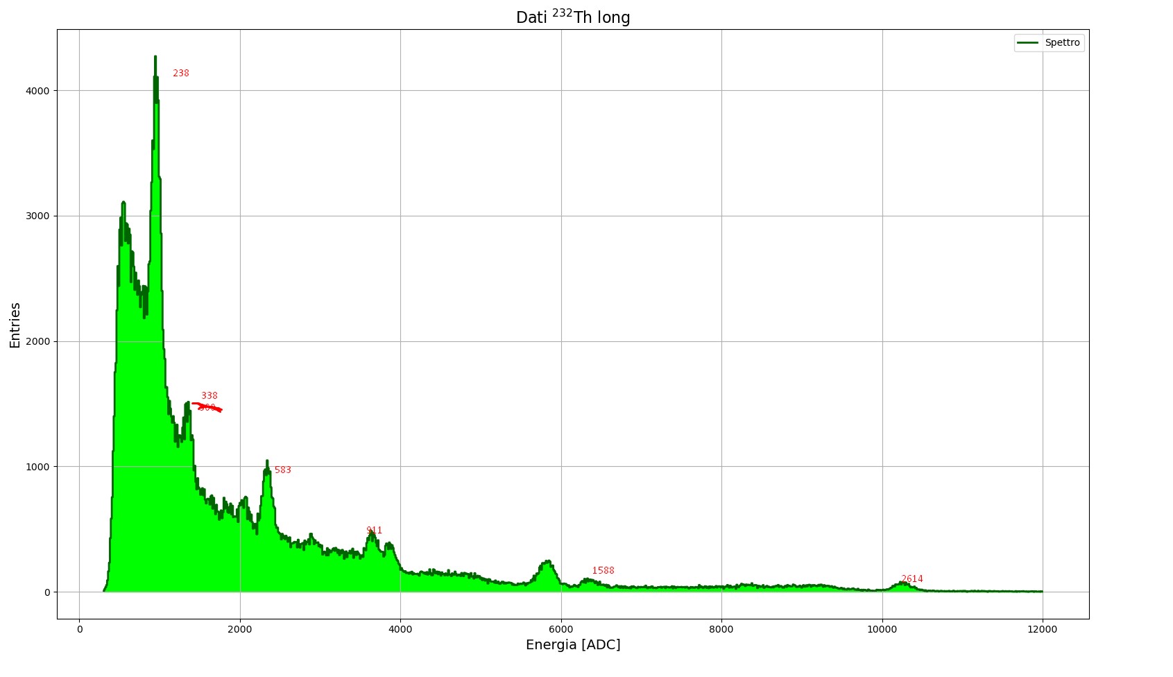
myRange = ((881, 1042), (1276, 1428), (2237, 2434), (3535, 3768), (6215, 6580), (10036, 10477))
energieVere = np.array((238, 338, 583, 911, 1588, 2614))

p0gaus = ((320703, 963.909, 52.8224),
          (28257.1, 1350.09, 37.0244),
          (28257, 2342, 100),
          
          (1e6, 3618, 175),
          (1e6, 6349, 200),
          (1e6, 10246, 300),
          )
p0exp = (33561.7, 0.00310716)
p0line = (-3.584035, 5222.718544)


def gaus(x,a,mu,sigma, b, c):
    return a/(sigma*np.sqrt(2*np.pi))* np.exp(-(x-mu)**2 / (2*sigma**2)) + b*x+c#+ b*np.exp(-c*x)

lstPopt = []
lstPcov = []

def fittaPicchi(idx, ax):
    
    ax = ax[idx]
    
    cond = (binc > myRange[idx][0]) & (binc < myRange[idx][1]) 
    
    popt, pcov = curve_fit(gaus, binc[cond], h[cond], sigma = np.sqrt(h[cond]), 
                           absolute_sigma = True, p0 = (*p0gaus[idx], *p0line))
    
    condPlot  =(binc > (myRange[idx][0]-200)) & (binc < (myRange[idx][1]+200)) 
    
    ax.plot(binc[condPlot], h[condPlot], ds = "steps-mid", c = "darkgreen", lw = 2, label = "Spettro")
    ax.fill_between(binc[condPlot], h[condPlot], step = "mid", color = "lime", alpha = 1)

    ax.plot(binc[cond], gaus(binc[cond], *popt), ls = "--", c = "k", lw = 2)
    
    lstPopt.append(popt)
    lstPcov.append(popt)


fig, ax = plt.subplots(3,2, dpi = 100)
fig.set_size_inches(12,5)
ax = ax.flatten()

for i in range(6): 
    fittaPicchi(i, ax)


plt.show()

Retta di calibrazione

In [10]:
lstPicchi = np.array([i[1] for i in lstPopt])
lstSigma = np.array([i[2] for i in lstPopt])

    
popt, pcov = curve_fit(line, energieVere, lstPicchi, sigma = lstSigma, absolute_sigma = True)


fig, ax = plt.subplots()
ax.errorbar(energieVere, lstPicchi, yerr = lstSigma, color = "tab:green", marker = "h", ls = "", ms = 3.5)
    
ax.plot(energieVere, line(energieVere, *popt), ":k")

ax.grid()
ax.set_xlabel("Energie vere [keV]", fontsize = 14)
ax.set_ylabel("Energie fittate [ADC]", fontsize = 14)
ax.set_title("Retta di calibrazione", fontsize = 16)


plt.show()

Spettro calibrato

In [11]:
m = 1/popt[0]
q = -popt[1]/popt[0]

bincE = line(binc, m, q)


fig, ax = plt.subplots()
fig.set_size_inches(12,5)

ax.plot(bincE, h, ds = "steps-mid", c = "darkgreen", lw = 2, label = "Spettro")
ax.fill_between(bincE, h, step = "mid", color = "lime", alpha = 1)


#ax.plot(binc, myFun(binc, *popt))

ax.grid()
ax.set_xlabel("Energia [keV]", fontsize = 14)
ax.set_ylabel("Entries", fontsize = 14)
ax.set_title("Dati $^{232}$Th long", fontsize = 16)
ax.legend()
#ax.set_yscale("log")

plt.show()
In [12]:
%matplotlib inline

def gaus(x,a,mu,sigma, b, c):
    return a/(sigma*np.sqrt(2*np.pi))* np.exp(-(x-mu)**2 / (2*sigma**2)) + b*x+c

cond = (bincE > 214) & (bincE < 255) 

popt, pcov = curve_fit(gaus, bincE[cond], h[cond], sigma = np.sqrt(h[cond]), 
                       absolute_sigma = True, p0 = (141202.843040, 236.924507, 16.782656, -1.5, 3000 ))

condPlot = (bincE > 133) & (bincE < 400) 

fig, ax = plt.subplots()

ax.plot(bincE[condPlot], h[condPlot], ds = "steps-mid", c = "darkgreen", lw = 2, label = "Spettro")
ax.fill_between(bincE[condPlot], h[condPlot], step = "mid", color = "lime", alpha = 1)

ax.plot(bincE[cond], gaus(bincE[cond], *popt), ls = "--", c = "b", lw = 3, label = "Curva fittata")


ax.grid()
ax.set_xlabel("Energia [keV]", fontsize = 14)
ax.set_ylabel("Entries", fontsize = 14)
ax.set_title("Dati $^{232}$Th - fit primo picco", fontsize = 16)
ax.legend()

plt.show()
In [13]:
print(f"La risoluzione vale {(235 * popt[2] / popt[1]):.2f} %")
La risoluzione vale 16.53 %

Cesio

In [14]:
nev, ts, qs, ql, ch = np.loadtxt("./DATI/LaBr3_Cs.txt", unpack = True, skiprows = 1)

h, bins = np.histogram(ql, bins = 1000, range = (300, 12000))
binc = bins[:-1] + (bins[1]-bins[0])/2

bincE = line(binc, m, q)
In [15]:
%matplotlib inline

def gausLine(x,a,mu,sigma, b, c):
    return a/(sigma*np.sqrt(2*np.pi))* np.exp(-(x-mu)**2 / (2*sigma**2)) + b*x+c

cond = (bincE > 611) & (bincE < 741) 
popt, pcov = curve_fit(gausLine, bincE[cond], h[cond], sigma = np.sqrt(h[cond]), absolute_sigma = True, p0 = [553335, 667.333, 15.4381, -10, 8000])

fig, ax = plt.subplots()
fig.set_size_inches(12,5)

ax.plot(bincE, h, ds = "steps-mid", c = "darkgreen", lw = 2, label = "Spettro")
ax.fill_between(bincE, h, step = "mid", color = "lime", alpha = 1)

ax.plot(bincE[cond], gausLine(bincE[cond], *popt), ls = "--", c = "k", lw = 3, label = "Curva fittata")

#ax.plot(binc, myFun(binc, *popt))

ax.grid()
ax.set_xlabel("Energia [ADC]", fontsize = 14)
ax.set_ylabel("Entries", fontsize = 14)
ax.set_title("Dati $^{137}$Cs long", fontsize = 16)
ax.legend()
#ax.set_yscale("log")

plt.show()
In [17]:
print(f"La risoluzione energetica per il cesio vale {235 * popt[2]/popt[1]:.1f} %")
La risoluzione energetica per il cesio vale 5.4 %

Per poster - [FOTO SPETTRO 137cS]

In [30]:
%matplotlib inline


fig, ax = plt.subplots()
fig.set_size_inches(12,5)

ax.plot(bincE, h, ds = "steps-mid", c = "darkgreen", lw = 2, label = "Spectrum")
ax.fill_between(bincE, h, step = "mid", color = "lime", alpha = 1)

ax.plot(bincE[cond], gausLine(bincE[cond], *popt), ls = "-", c = "b", lw = 3, label = "Fitted curve (gauss + p1)")

#ax.plot(binc, myFun(binc, *popt))

ax.grid()
ax.set_xlabel("Energy [keV]", fontsize = 14)
ax.set_ylabel("Entries", fontsize = 14)
ax.set_title("$^{137}$Cs spectrum", fontsize = 16)
ax.legend()
ax.set_yscale("log")
ax.set_xlim((0, 2000))

plt.show()

Run di più giorni (Torio)

In [15]:
nev, ts, qs, ql, ch = np.loadtxt("./DATI/LaBr3_232Th_runPiuGiorni.txt", unpack = True, skiprows = 1)

h, bins = np.histogram(ql, bins = 1000, range = (300, 12000))
binc = bins[:-1] + (bins[1]-bins[0])/2

#bincE = line(binc, m, q)
In [16]:
%matplotlib inline
#%matplotlib qt


fig, ax = plt.subplots()
fig.set_size_inches(12,5)

ax.plot(binc, h, ds = "steps-mid", c = "darkgreen", lw = 2, label = "Spettro")
ax.fill_between(binc, h, step = "mid", color = "lime", alpha = 1)


#ax.plot(binc, myFun(binc, *popt))

ax.grid()
ax.set_xlabel("Energia [ADC]", fontsize = 14)
ax.set_ylabel("Entries", fontsize = 14)
ax.set_title("Dati $^{232}$Th più giorni", fontsize = 16)
ax.legend()
#ax.set_yscale("log")

plt.show()
In [17]:
ql.shape
Out[17]:
(15392863,)